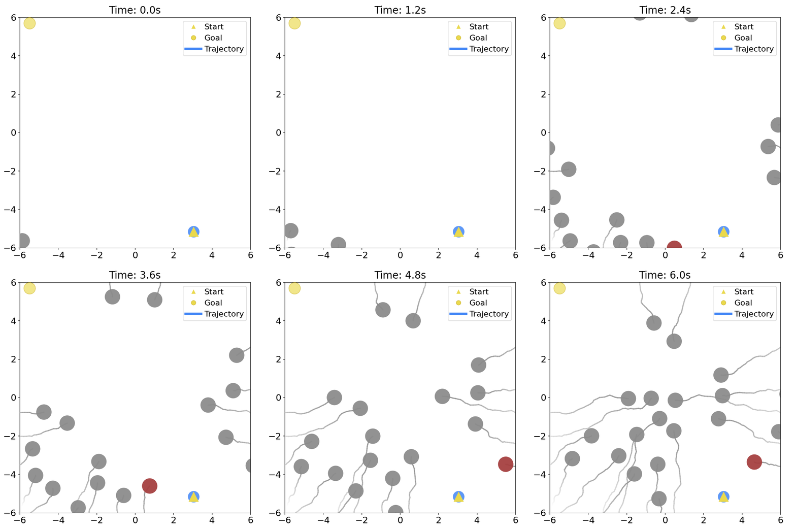
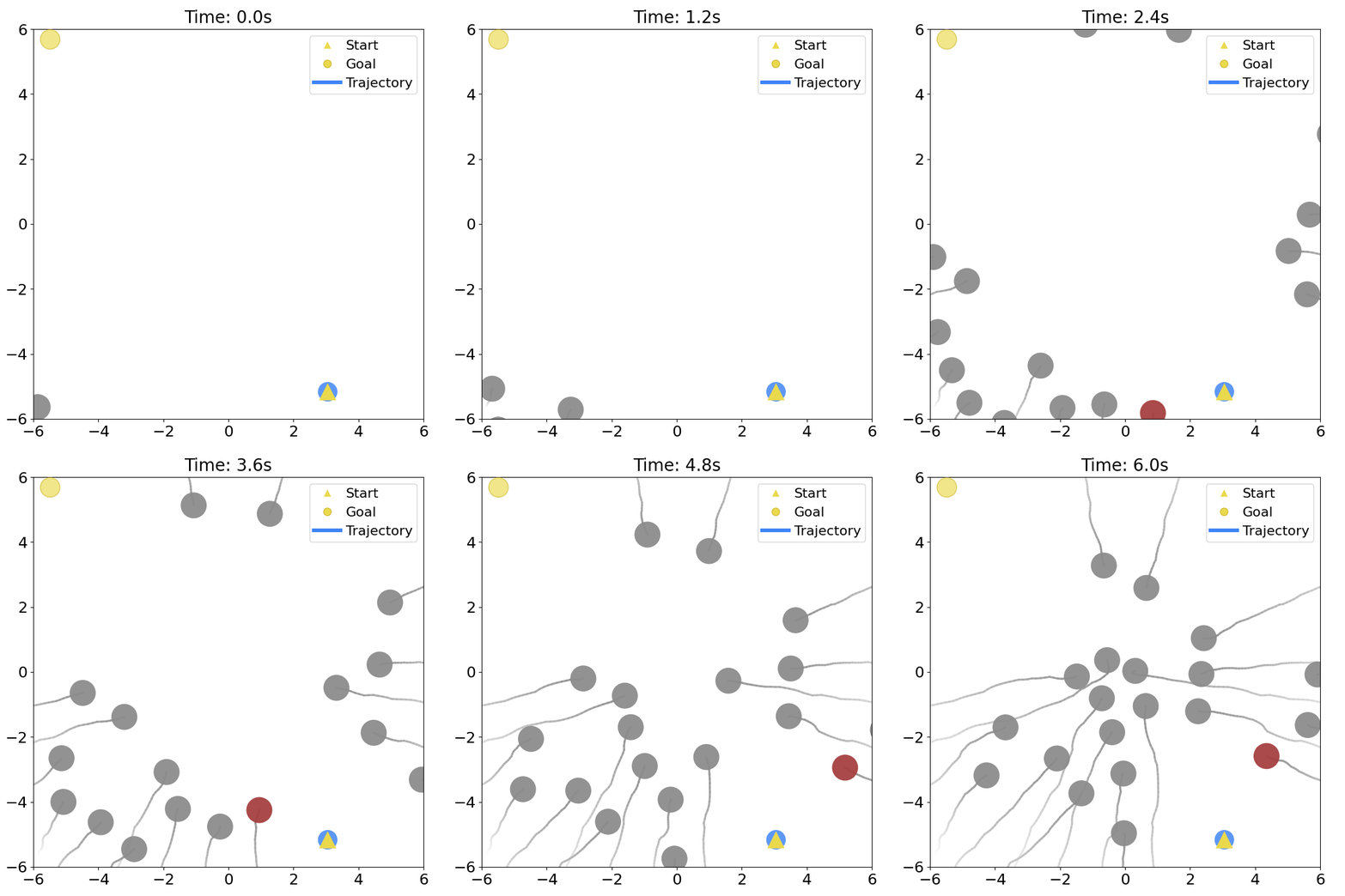
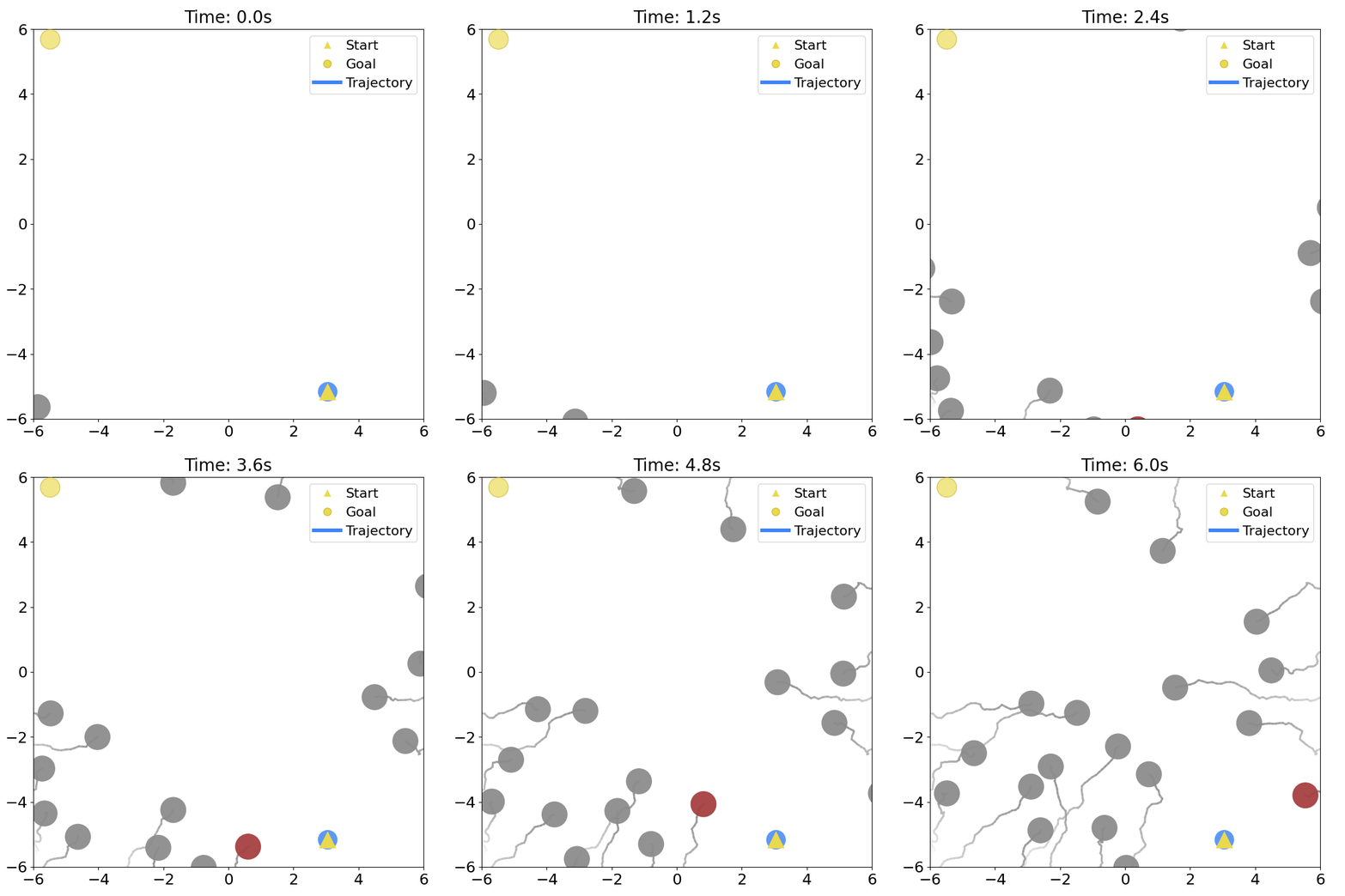
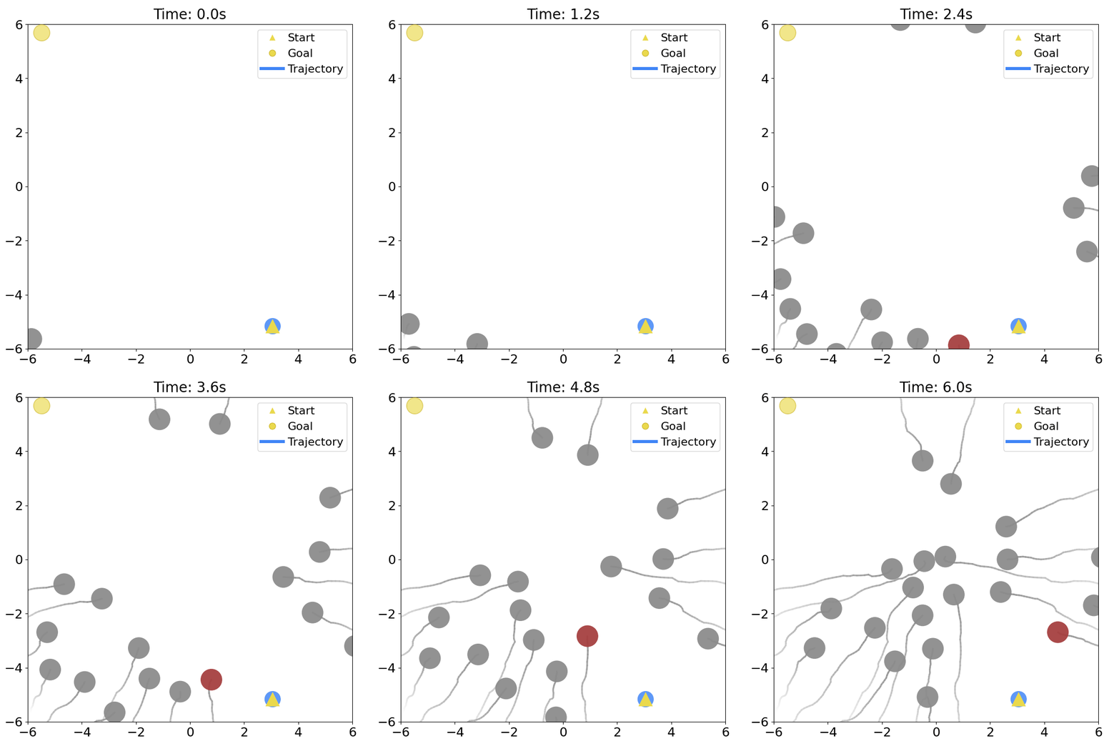
Risk Adaptation Settings In-Distribution Demos Out-of-Distribution Demos Statistical Results

Reinforcement Learning for Risk Adaptation via Differentiable CVaR Barrier Functions

Anonymous

TL;DR

Learning to adapt risk online is critical for navigation in uncertain crowds. We present an end-to-end risk-adaptive framework that combines reinforcement learning with a differentiable CVaR barrier-function safety layer, jointly learning nominal control, risk level, and safety margin while enforcing probabilistic safety guarantees. This lets the robot stay cautious in difficult interactions without becoming unnecessarily conservative, and it performs strongly across varying obstacle densities, robot models, and OOD crowd shifts.

Method Overview

Method Overview Figure

Simulation Settings

01

Environment & Uncertainty

Workspace
[-6, 6] × [-6, 6] m
Obstacles
20 dynamic circles; radius 0.4 m; speed in [0.5, 1.5] m/s
Human motion
Social-force policy with avoid_robot = false
Uncertainty
Three-mode GMM; weights [0.6, 0.2, 0.2], standard deviations [0.1, 0.2, 0.2], lateral ratio 0.3
02

Robot & Control

Dynamics
Single-integrator and unicycle; robot radius 0.3 m
Single-integrator
||u|| ≤ 1.5 m/s
Unicycle
v ∈ [-1.5, 1.5] m/s; ω ∈ [-1.57, 1.57] rad/s
Simulation
Δt = 0.1 s; 400 steps per episode; goal tolerance 0.6 m
Observation
20 m sensing range with three-frame history
03

QP

Policy output
unom,k, {βi,k}, and {ΔRi,k}
Risk allocation
Total budget 0.5 with βmin = 0.05
Safety margin
Base margin 0.05 m; maximum adaptive increment 1.125 m
QP parameter
Class-K gain α = 2.0
Solver
Differentiable JAX qpth QP layer with slack weight 10.0
04

Evaluation Protocol

Final statistics 10 base seeds × 50 episodes
Episode horizon 40 s (400 steps)
OOD conditions 30 obstacles and obstacle radius increased to 0.5 m

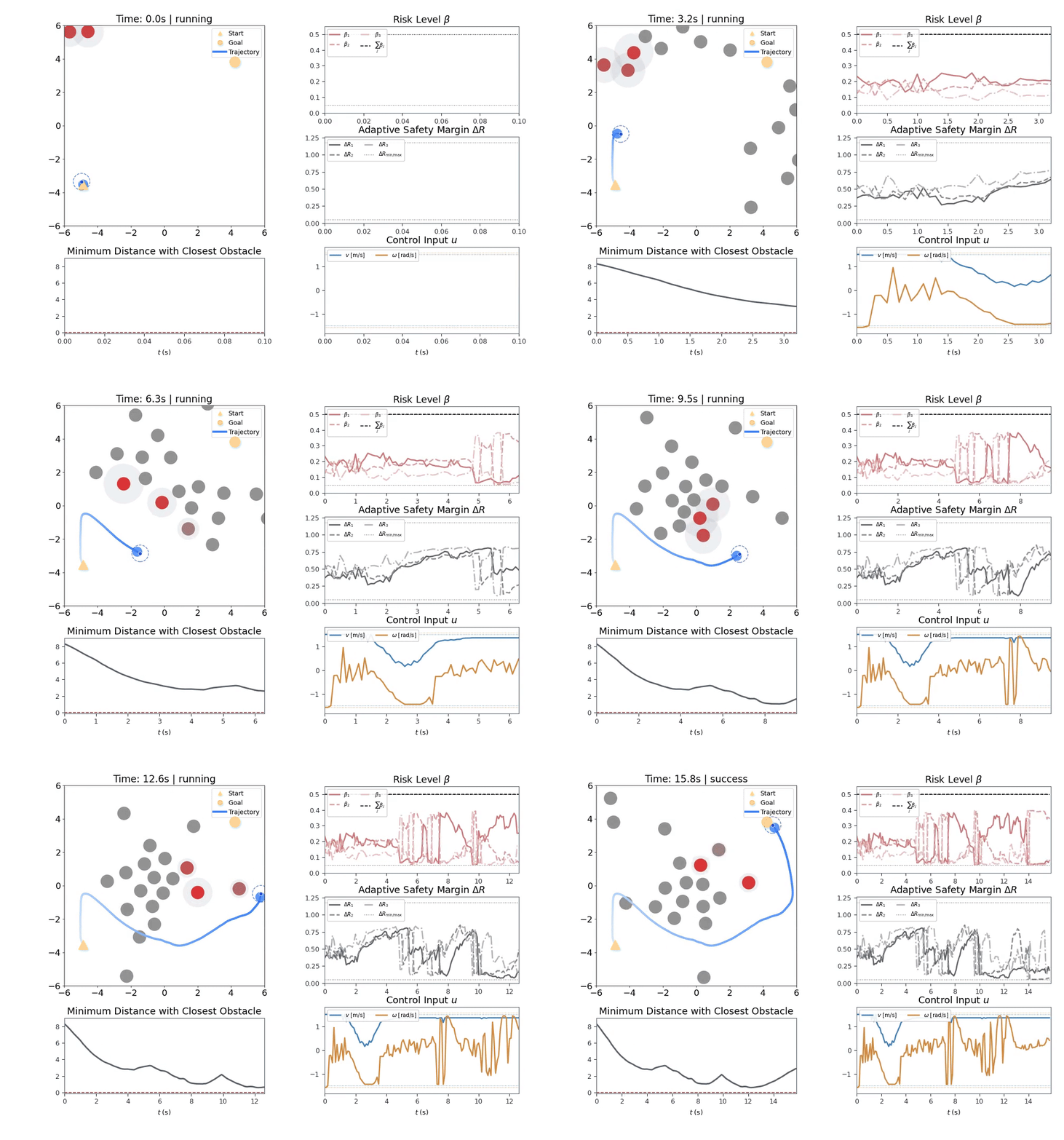
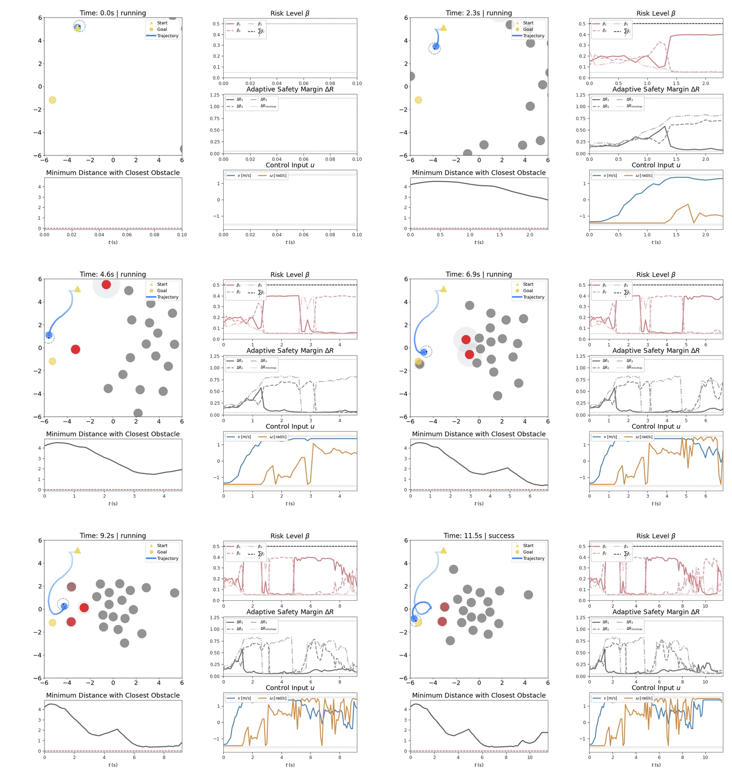
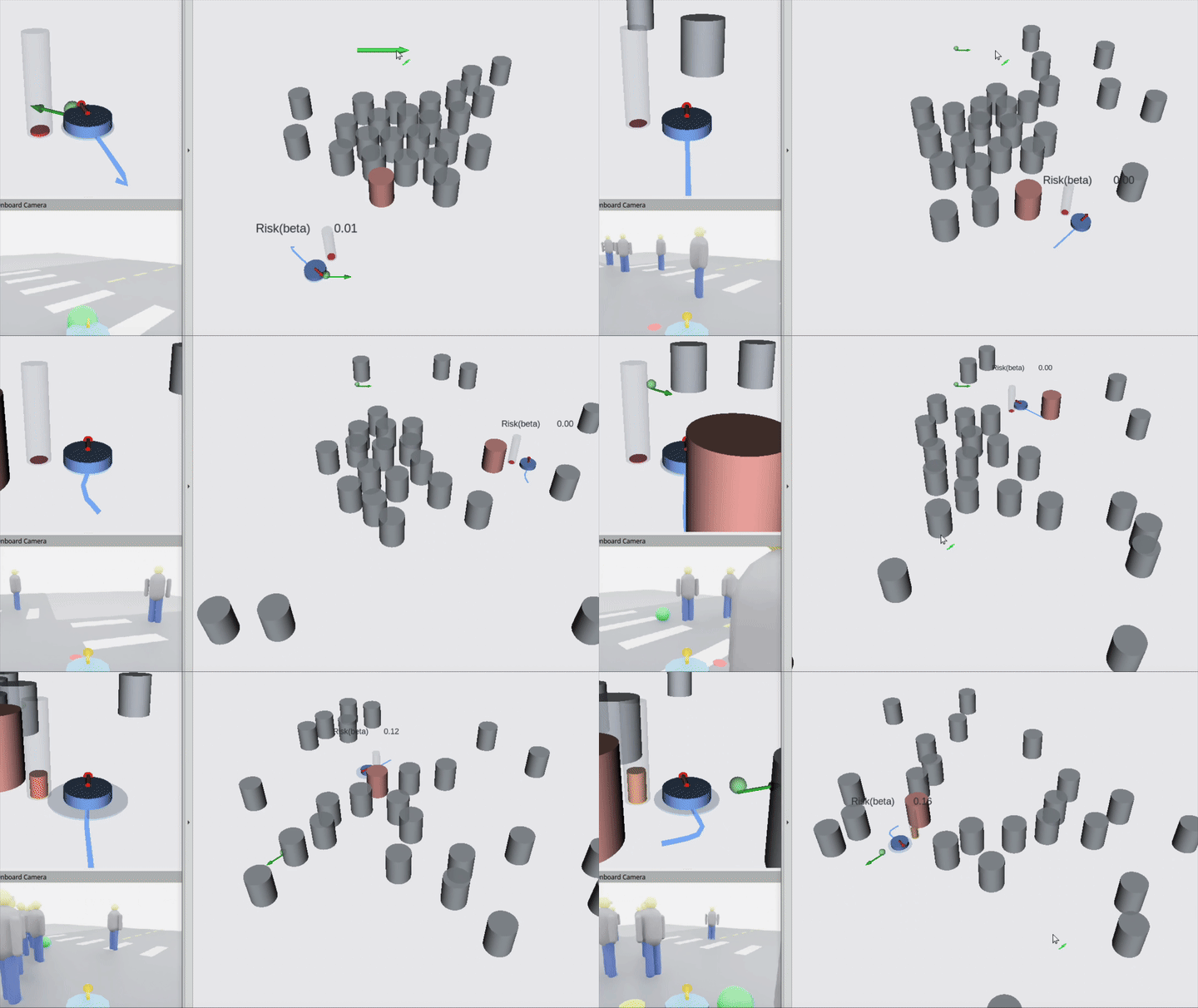
In-Distribution Demos

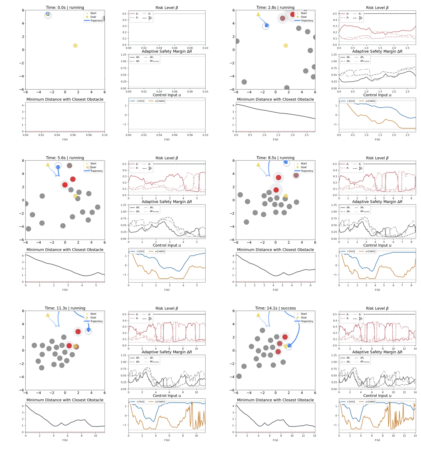
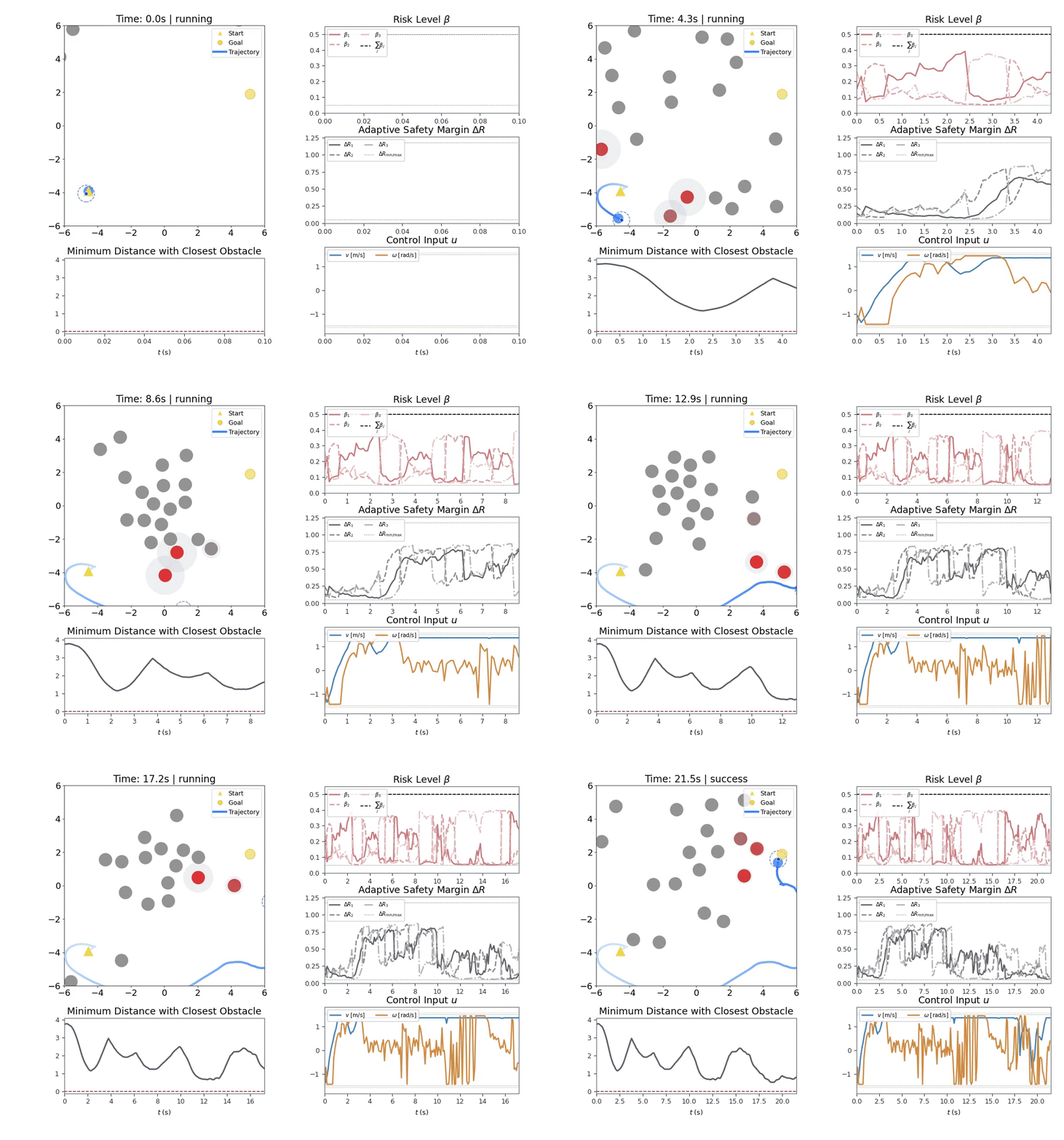
Out-of-Distribution Demos

Compared Methods

We compare optimization-based controllers, learned navigation policies, and hybrid safety-filtered methods.

Optimization

ORCA, CBF-QP, CVaR-BF-QP, and Adaptive-CVaR-BF-QP

Reinforcement Learning

Vanilla RL and CrowdNav++ with constant-velocity or inferred obstacle motion

RL + Optimization

Safety-filtered RL variants, BarrierNet, and the proposed Diff-CVaR-GNN

Statistical Results

Table I baseline comparison for the single-integrator model in a 20-obstacle environment
Table I(a) — Single-integrator
Table I baseline comparison for the unicycle model in a 20-obstacle environment
Table I(b) — Unicycle
Success rate versus obstacle count for the unicycle model
Unicycle
Q1: How do different method types compare in dynamic environments?
  • RL + Optimization: best safety & efficiency.
  • Optimization only: lower success rate due to infeasibility.
  • RL only: efficient but no formal safety guarantee.
Q2: How do different ways of integrating safety into RL affect performance?
  • End-to-end training: outperforms decoupled post-hoc safety filtering.
  • Joint learning eliminates the optimality gap.
  • Outperforms BarrierNet by modeling stochastic uncertainty.
Q3: How robust are all methods across obstacle densities?
  • Proposed method: most robust among others, with graceful degradation.
  • Obstacle Density: degrade gracefully.
Table II out-of-distribution generalization for the unicycle model. Case I uses 30 obstacles; Case II increases the obstacle radius to 0.5 meters
Table II — Unicycle
Case I: high obstacle density (30 obstacles). Case II: increased obstacle radius (0.5 m).
Q4: How robust are different type of methods under OOD environment changes?
  • Proposed method: adaptation gives best OOD success rate.
  • RL only: degrades most under unseen policy shifts.
  • RL + Safety Filter: regains robustness but still lags behind.
Setting Weights [w1, w2, w3] Stds [σ1, σ2, σ3] Lat.
Matched / oracle GMM [0.6, 0.2, 0.2] [0.1, 0.2, 0.2] 0.3
A.1 Policy overestimates uncertainty [0.8, 0.1, 0.1] [0.05, 0.1, 0.1] 0.2
A.2 Policy underestimates uncertainty [0.4, 0.3, 0.3] [0.2, 0.4, 0.4] 0.4
B Imbalanced mode weights [0.9, 0.05, 0.05] [0.1, 0.2, 0.2] 0.3

GMM parameter settings. The policy keeps the matched/oracle belief fixed while the environment parameters change. Lat. denotes the lateral-mode displacement ratio.

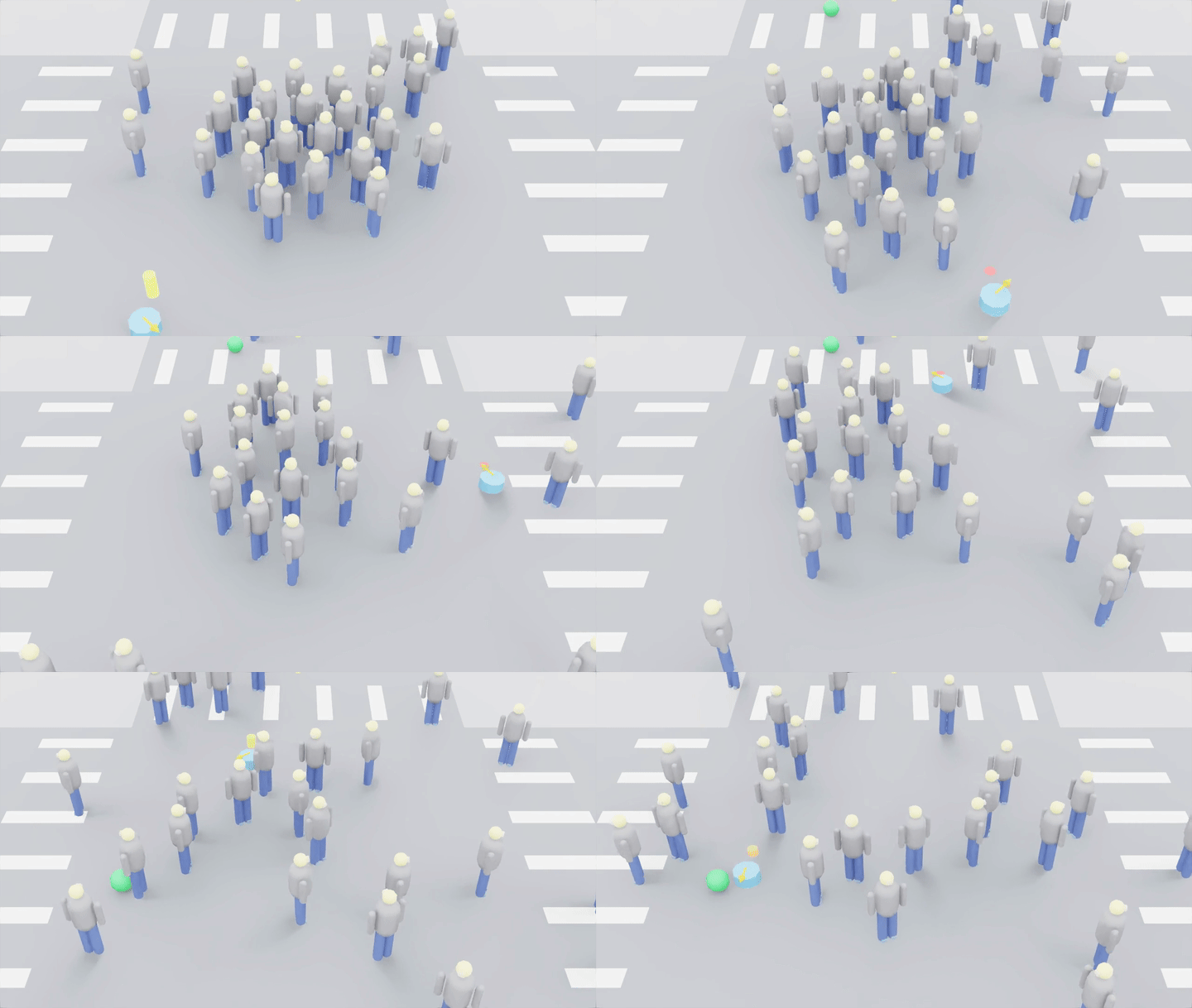
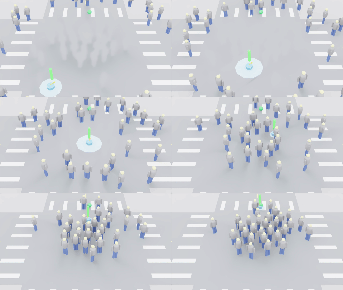
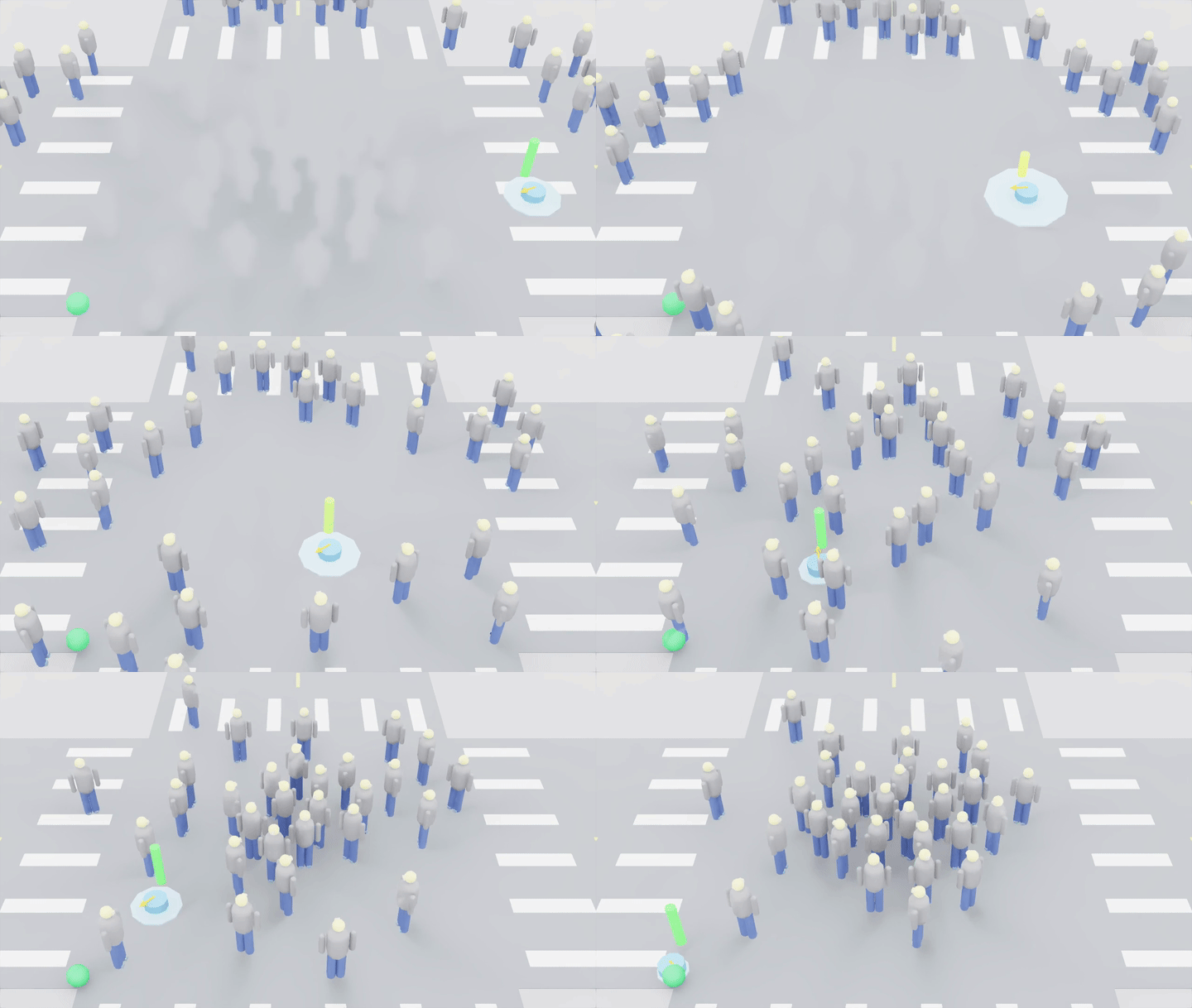
GMM trajectory examples

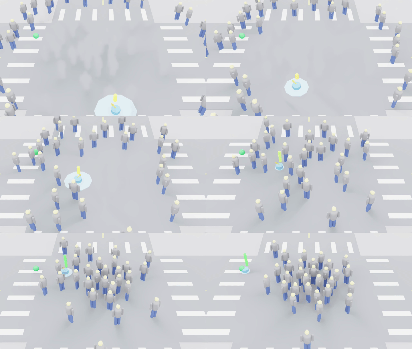
All animations use the same reset seed and a fixed policy; only the environment GMM changes. The matched/oracle animation is the common baseline for both groups.

Group A — uncertainty mismatch

Six-second environment trajectory animation for the matched oracle GMM
A.0 Matched / oracle GMM
Six-second environment trajectory animation when the policy overestimates GMM uncertainty
A.1 Policy overestimates uncertainty
Six-second environment trajectory animation when the policy underestimates GMM uncertainty
A.2 Policy underestimates uncertainty

Group B — mode-weight mismatch

Six-second environment trajectory animation for the matched oracle GMM baseline in Group B
B.0 Matched / oracle GMM
Six-second environment trajectory animation for imbalanced GMM mode weights
B.1 Imbalanced mode weights
GMM Setting Success Rate (%) Collision Rate (%)
Matched / oracle GMM 97.0 2.6
A.1 Policy overestimates uncertainty 97.4 2.4
A.2 Policy underestimates uncertainty 92.4 6.2
B Imbalanced mode weights 96.8 2.6

Table III — Unicycle
Q5: How robust is the method to GMM mismatch?
  • The method shows empirical robustness to moderate GMM mismatch, with graceful degradation when uncertainty is underestimated.
Ablation study of adaptive risk allocation, adaptive safety margin, and the safety layer for the unicycle model
Table IV — Unicycle
Policy 1: full; Policy 2: fixed risk; Policy 3: fixed margin; Policy 4: both fixed; Policy 5: no safety layer.
Q6: How does each adaptive component affect performance?
  • Each adaptive component contributes: the full method achieves 97.0% SR and 2.6% CR, while removing the safety layer causes the largest degradation.

Real-Time Safe Navigation

Real-time safe navigation with ROS 2
Real-time safe navigation in Isaac Sim